| Generative (i.e., Classical Statistics) | |||
|---|---|---|---|
| Predictive (i.e., Machine Learning) | |||
Machine Learning
A Gentle Introduction
Supervised Machine Learning (SML)
Once deployed, SML algorithms learn the complex patterns linking \(X\)—a set of features (or independent variables)—to a target variable (or outcome), \(Y\).
The goal of SML is to optimize predictions—i.e., to find functions or algorithms that offer substantial predictive power when confronted with new or unseen data.
Examples of SML algorithms include logistic regressions, random forests, ridge regressions and neural networks.
A quick note on terminology
If a target variable is quantitative, we are dealing with a regression problem.
If a target variable is qualitative, we are dealing with a classification problem.
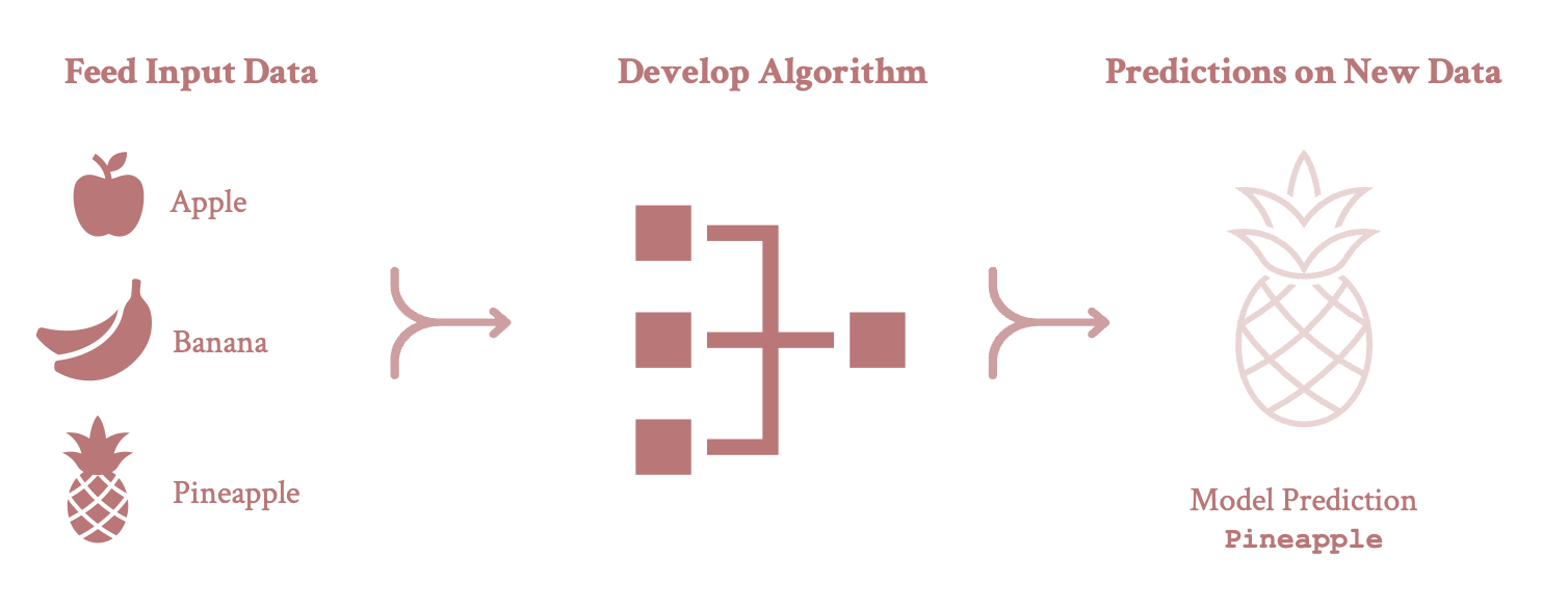
Note: This figure is an adaptation of the diagram depicted here
Unsupervised Machine Learning (UML)
UML techniques search for a representation of the inputs (or features) that is more useful than \(X\) itself (Molina and Garip 2019).
- Put another way, UML algorithms search for hidden structure in high dimensional space.
In UML, there is no observed \(Y\) variable—or target—to supervise the estimation process. Instead, we only have a vector of inputs to work with.
The goal in UML is to develop a lower-dimensional representation of complex data by inductively learning from the interrelationships among inputs.
- This can be achieved by reducing a vector of features to a smaller set of scales (e.g., via principal component analysis) or partitioning the sample into a small number of unobserved groups (e.g., via k-means clustering).


Bias-Variance Tradeoff
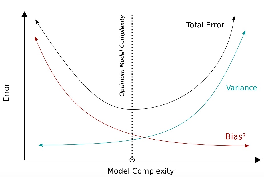
Image can be retrieved here.
Bias emerges when we build SML algorithms that fail to sufficiently map the patterns—or pick up the empirical signal–linking \(X\) and \(Y\). Think: underfitting.
Variance arises when our algorithms not only pick up the signal linking \(X\) and \(Y\), but some of the noise in our data as well. Think: overfitting.
When adopting an SML framework, researchers try to strike the optimal balance between bias and variance.
\(k\)-Fold Cross-Validation
Unlike conventional approaches to sample partition, \(k\) or \(v\)-fold cross-validation allows us to learn from all our data.
\(k\)-fold cross-validation proceeds as follows:
- We randomly divide our overall sample into \(k\) subsets or folds.
- We train our algorithm on \(k - 1\) folds, holding just one group out for model assessment.
- We repeat this process \(k\) times—every fold is held out once and used to fit the model \(k - 1\) times.
- We then pool or average the evaluation metrics (e.g., predictive accuracy) for all the held-out runs.
Stratified \(k\)-fold cross-validation ensures that the distribution of class labels (or for numeric targets, the mean) is relatively constant across folds.
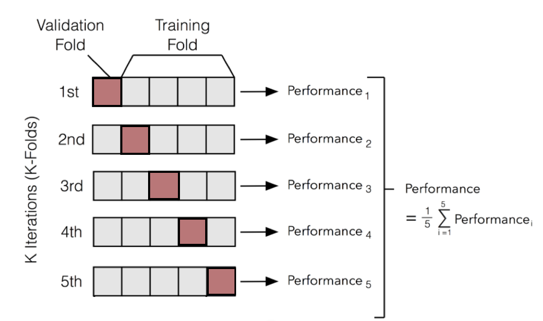
Image can be retrieved here.